Monopolar RF Thermal Dispersion Model for the Vaginal Wall

Catalog of Regulatory Science Tools to Help Assess New Medical Devices

Technical Description

The Monopolar RF Thermal Dispersion Model for the Vaginal Wall provides vaginal thermotherapy (VTT) device designers with a first-pass estimation of the thermal effect produced in the vaginal wall by their device. Finite element analysis (FEA) was used to calculate the energy deposition due to radio frequency (RF) exposure and the bioheat transfer field simultaneously.

This tool should be used as a screening-level check on the depth of thermal dispersion for a device design and protocol, specifically that the device is only heating the target tissue and not heating deeper than the target tissue. If the device is heating past the target tissue, it could be unintentionally affecting sensitive adjacent tissue, such as the urethra. The device designer may use these data to inform their design process. This tool is meant to supplement in vivo or in vitro experiments and not as a stand-alone safety assessment tool.

The tool was originally implemented in COMSOL Multiphysics using the AC/DC and Heat Transfer Modules.

User inputs:

• Probe size and shape
• RF power
• Exposure time
• Probe tip cooling condition

Tool outputs:

• Area of thermal effect
• Depth of thermal dispersion marked by 43˚C isotherm
• Thermal field visualization in layered tissue section
• Comparison of deepest thermal extent to minimum vaginal wall boundary

Intended Purpose

This tool is designed to model a subset of vaginal thermotherapy devices which use monopolar radiofrequency (RF) only to heat the vaginal wall. This tool is not applicable to bipolar or multipolar RF devices or to laser-based vaginal heat therapy devices.

Ensuring the energy deposition and resultant heating is confined to the vaginal wall is intended to help ensure the safety of these devices. The purpose of this FEA-based tool is to provide device designers with an approximation of the depth of heating for their monopolar RF VTT devices. If the simulated area of thermal effect penetrates past the vaginal wall boundary, the device designers can iteratively change input parameters to address the issue.

FEA provides a rapid and flexible precursor to any follow-up benchtop experiments on ex vivo or in vivo tissue.

This tool should be implemented by a user with experience in FEA or similar numerical simulation techniques. The simulations were originally performed in COMSOL Multiphysics, but can be implemented in a number of FEA platforms using the simulation setup information provided in the Step-by-step user guide below.

This tool is meant to supplement in vivo or in vitro experiments and not as a stand-alone safety assessment tool.

Testing

This model is intended for screening-level usage, and not to be used in place of in vivo or in vitro models.

Validation details are provided in section 12 of the step-by-step user guide and in Ian A Carr et al 2021 Biomed. Phys. Eng. Express 7 065022. Depth of thermal dispersion of monopolar radiofrequency heating in the vaginal wall - IOPscience.

User-specific validation will be required based on the context of use (CoU) of the model and the associated model risk as defined by the user. Please refer to Sections 3 and 4 of ASME V&V40-2018, "Assessing Credibility of Computational Modeling through Verification and Validation: Application to Medical Devices" for additional details about CoU and model risk.

Limitations

Biological tissue has inherent inter- and intra-patient variation in material properties and geometry. As such, the results output by this tool should be considered a first-pass approximation of the area of thermal dispersion. The tool is designed to give a conservative estimate of the area of thermal effect. This tool is meant to supplement in vivo or in vitro experiments and not as a stand-alone safety assessment tool.

Supporting Documentation

See step-by-step user guide in Appendix below.

Contact

• RST_CDRH@fda.hhs.gov

Tool Reference

 In addition to citing relevant publications please reference the use of this tool using DOI: 10.5281/zenodo.7558824.

For more information:

• Catalog of Regulatory Science Tools to Help Assess New Medical Devices

---

Appendix: Step-by-step instructions

Numerically simulating monopolar radiofrequency-based vaginal thermotherapy

1. Software Requirements

This guide was developed using COMSOL Multiphysics version 5.5. If another version is used some features or processes may differ. The user of this guide is responsible for determining how to implement the steps in this guide in a different version of COMSOL Multiphysics or other simulation software. If the user intends to use other software refer to the following manuscript for a conceptual discussion of the process along with the accompanying equations.

• Carr IA, Garcia M, Cordray D, Lee A, Shrivastava D, Hariharan P. Depth of thermal dispersion of monopolar radiofrequency heating in the vaginal wall. Biomed Phys Eng Express. 2021 Oct 5;7(6). doi: 10.1088/2057-1976/ac28ac. PMID: 34547744.

If using COMSOL Multiphysics, the user is required to have the AC/DC and Heat Transfer Modules to follow the steps of this guide exactly. There are ways to implement the same equations via user-defined equations but that is outside the scope of this guide.

2. Model Initiation

• Open COMSOL Multiphysics
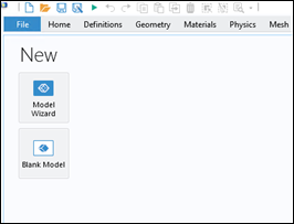
• Initiate the Model Wizard

• Under Select Space Dimensions, Select a 3D model space

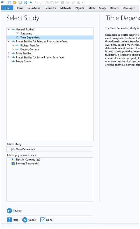
• Under Select Physics, Select the following modules:
  AC/DC –> Electrical Fields and Currents –> Electrical Currents
  Heat Transfer –> Bioheat Transfer
• Click Study

• Under Select Study, Select a Time Dependent Study
• Hit Done

A. Define Independent Parameters

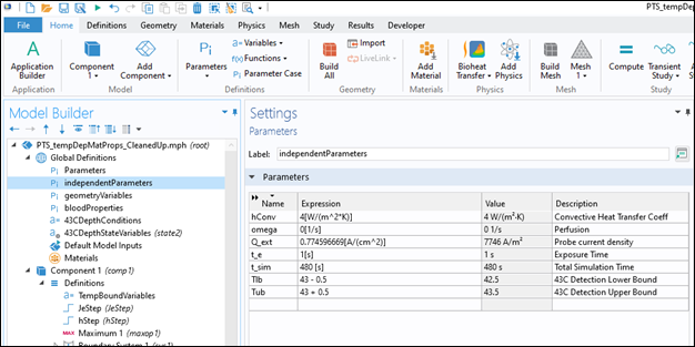
• Once the model space is open, define a set of parameters using Global Definitions. Right click on Global Definitions and open a new parameter group.

Note: The values shown in the table below are those used in Carr et al (2021). The users of this guide may change these values depending on the use case of their simulation.
Either define those of your choosing or, to recreate the published simulations exactly, use the following:

Name	Expression	Description
hConv	4[W/(m^2*K)]	Convective Heat Transfer Coeff
omega	0[1/s]	Perfusion
Q_ext	0.774596669[A/(cm^2)]	Probe Current Density
t_e	1[s]	Exposure Time
t_sim	480[s]	Total Simulation Time
Tlb	43 - 0.5	43C Detection Lower Bound
Tub	43 + 0.5	43C Detection Upper Bound

B. Define Geometry Parameters

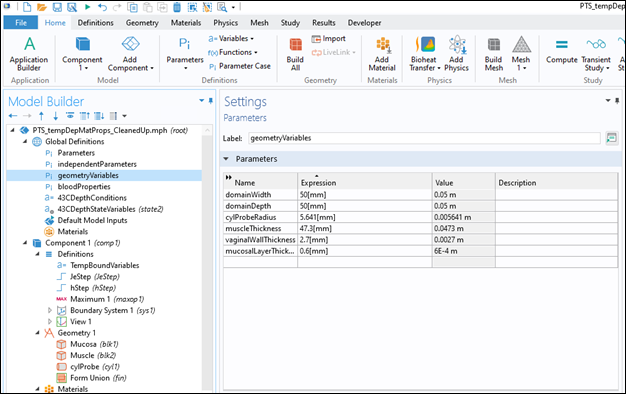
• Similarly, define a set of geometry parameters by right clicking Global Definitions and selecting Parameters

Note: Defining the geometry parameters this way is optional but can be a helpful organizational technique for later modification of the model geometry.

domainWidth	50[mm]
domainDepth	50[mm]
cylProbeRadius	5.641[mm]
muscleThickness	47.3[mm]
vaginalWallThickness	2.7[mm]

C. Define D43 Detection Variables

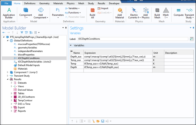
Next, we define a set of parameters and state variables to allow for the detection of the depth of the 43C isotherm – the chosen indicator of the depth of thermal dispersion. The results of this can be seen in D43 vs Time under the Results section below.

• Right click Global Definitions and select Variables and input the following:

Name	Expression	Unit
Depth_aux	comp1.maxop1(comp1.at3(25[mm],25[mm],z,T*aux_var),z)	m
Temp_aux	comp1.maxop1(comp1.at3(25[mm],25[mm],z,T*aux_var))	K
Temp	if(Temp_aux==0,NaN,Temp_aux)	K
Depth	if(Temp_aux==0,NaN,Depth_aux)	m

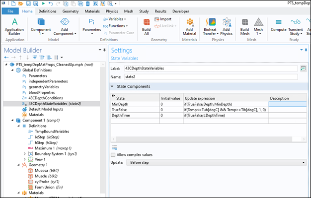
• Next a set of conditions as part of the automated detection of the 43C isotherm by right clicking Global Definitions and selecting Variables

Name	Initial value	Update Expression
minDepth	0	if(TrueFalse,Depth,MinDepth)
Temp_aux	0	if(Temp<=Tub[degC] && Temp>=Tlb[degC],1,0)
Temp	0	if(TrueFalse,t,DepthTime)

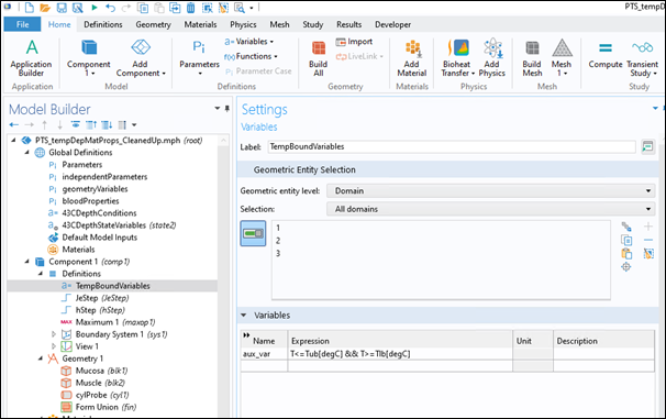
• Moving down to Component 1 define a similar auxiliary expression by right clicking Definitions and selecting Variables and defining the following:

Name	Expression
aux_var	T<=Tub[degC] && T>=Tlb[degC]

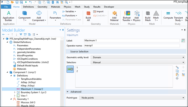
• Define maximum operator to detect the maximum temperature within the domain by right clicking Definitions in Component 1 then selecting Nonlocal Coupling then Maximum

D. Define Time-Dependent Variable Conditions Within Component 1

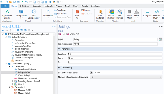
• Define step which reduces input power to 0 at the end of the exposure time by right clicking Definitions then selecting Functions then Step and inputting the variables as below

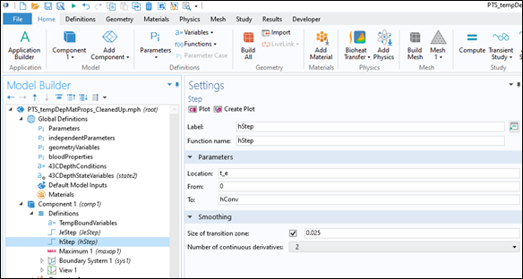
• Similarly, define a step condition to transition the convective heat transfer coefficient from 0 to the defined value. This simulates the removal of the probe from the tissue surface.

3. Building Geometry

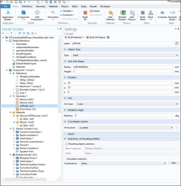
There are three parts of geometry to build to represent the model vaginal wall cross section – the mucosal layer, the muscular layer, and the probe itself. The geometry presented in this guide is meant to represent a generic device. If a specific device is being modeled the user may need to modify the geometry.

Note: In the coordinate system used herein the surface of the vaginal wall is z=0.

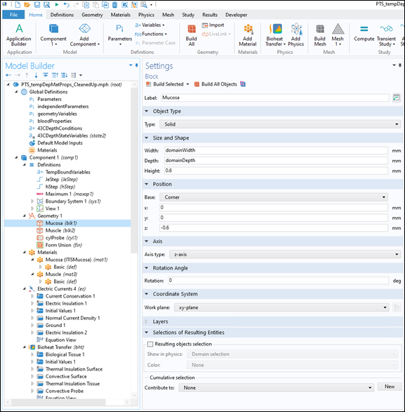
• Build the mucosal layer. Some of the dimensions are defined in Global Definitions herein. This is optional. The parameters should be input as they are below.
• Right click Geometry, select Block

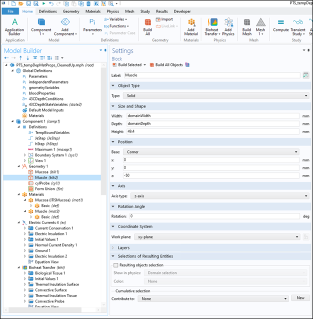
• Build the muscle layer with the dimensions below by right clicking Geometry and selecting Block and defining the dimension and position as follows.

• Build the probe geometry by right clicking Geometry then select Cylinder and inputting the size and position as below.

4. Assigning Material Properties

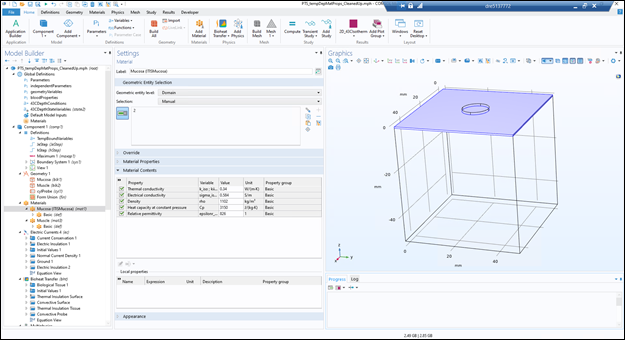
A. Assign Mucosal Material Properties

• Create a new material group by right clicking Material then selecting Blank Material then naming the group.
• Input the required material properties as below. Note: these material properties were those used in Carr et al 2021 but can change on a case-by-case basis

Property	Variable	Value	Unit	Property Group
Thermal Conductivity	k_...	0.34	W/mK	Basic
Electrical Conductivity	sigma_...	0.584	S/m	Basic
Density	rho	1102	Kg/m3	Basic
Heat Capacity	Cp	3150	J/kgK	Basic
Relative Permittivity	epsilon…	826	1	Basic

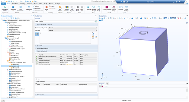
B. Assign Muscle Material Properties

• Assign the muscle material to the muscular layer using the same process and assign the material properties below.

Note: In this we used a temperature dependent material property for the electrical conductivity. This may increase the validity of your results but should be considered on a case-by-case basis.

Property	Variable	Value	Unit	Property Group
Heat Capacity	k_...		W/mK	Basic
Density	sigma_...	0.584	S/m	Basic
Density	rho	1102	Kg/m3	Basic
Heat Capacity	Cp	3150	J/kgK	Basic
Relative Permittivity	epsilon…	826	1	Basic

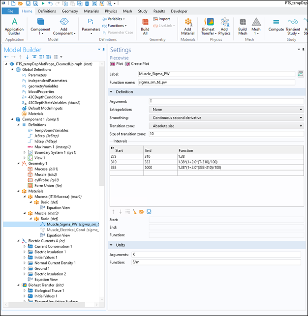
C. Define Temperature Dependent Material Properties

• Define the temperature dependent material. Under the Muscle material property right click Basic then Functions then Piecewise and enter the material property functions as below.

5. Assigning Boundary and Initial Conditions

A. Electrical Currents

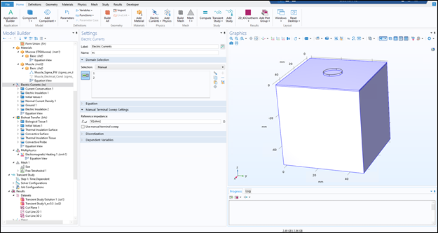
• Assign a reference impedance of 50 Ohms within Electrical Currents and assign it to the entire domain by selecting the volume in the Graphics window. The result should be as shown below

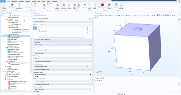
• Assure Current Conservation is assigned to the entire tissue volume (excluding the probe). This is the default setting and should be ready without modification.

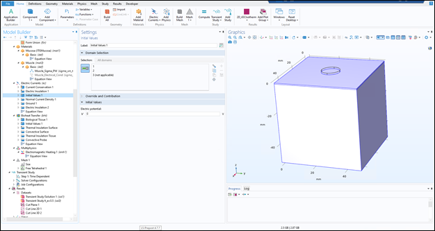
• Assign the Initial Values to 0V in the entire tissue domain (excluding the probe). The result should be visualized as below.

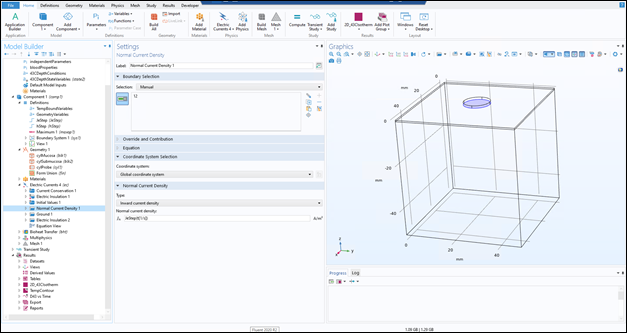
• Initiate and assign a Normal Current Density boundary condition to the probe-mucosal surface interface. If the mouse is hovering over multiple planes use the scroll wheel to choose which of the planes is selected.
• Use the JeStep(t[1/s]) step condition to assign the chosen current density (in Independent Parameters) to the probe-mucosal surface interface for the duration of exposure time (t_e). After t_e the current density set to 0. The visualization should appear as below.

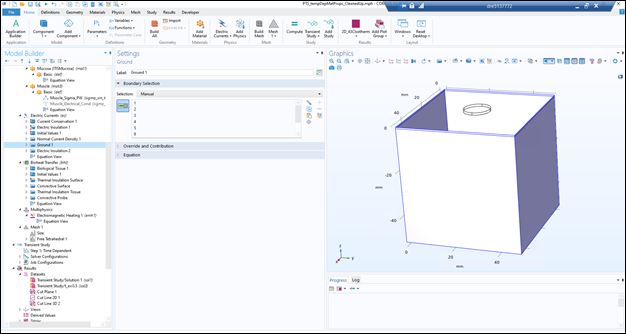
• Assign a Ground boundary condition to the sides and base of the two tissue layers. Assure that the narrow side walls of the mucosal layer are selected.

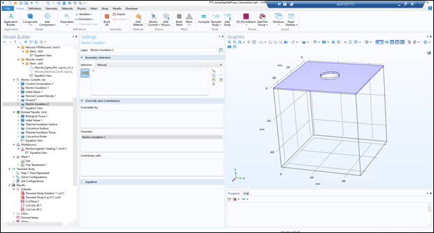
• Assign an Electrical Insulation boundary condition to the upper surface of the mucosal layer as below.

B. Bioheat Transfer

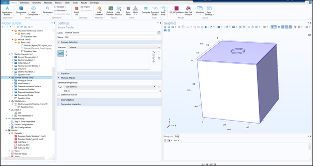
• Assign the Bioheat Transfer module to the entire domain as below.

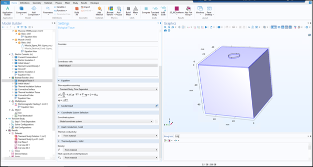
• Assign the Biological Tissue condition to the tissue domain by right clicking Bioheat Transfer then Specific Media then Biological Tissue

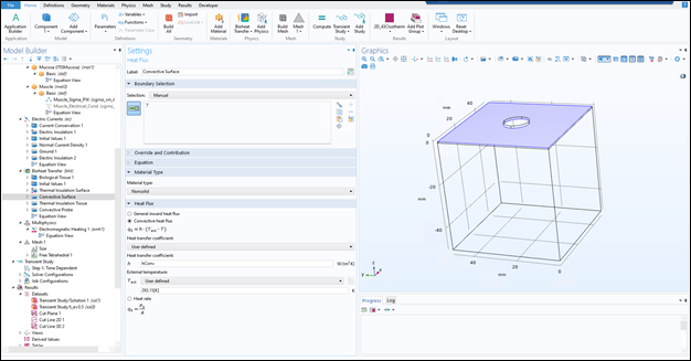
• Assign a convective condition to the exposed upper surface of the mucosal layer by right clicking Bioheat Transfer then Heat Flux then configuring as below. Exclude the probe tip, its boundary condition requires a step change condition.

• Assign a Thermal Insulation boundary condition to all tissue surfaces excluding the top surface and probe interface by right clicking Bioheat Transfer then Thermal Insulation and assigning to the proper surfaces.

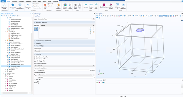
• Assign the convective heat transfer condition to the probe surface by right clicking Bioheat Transfer then Heat Flux then assign the step condition defined in Section 2D as shown below.

This condition uses a step change to transition the convective heat transfer coefficient from 0 to the same value assigned as the surrounding tissue. This simulates the removal of the probe from the tissue exposing the tissue to the same convective condition as the surrounding tissue.

6. Multiphysics Coupling

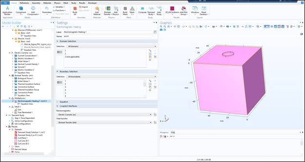
• Assure that the Multiphysics coupling, electromagnetic heating, is applied to the entire domain as below.

7. Meshing

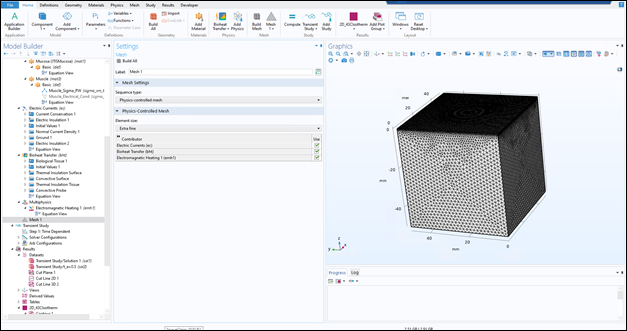
• Apply meshing to the entire domain. The density of the mesh dictates the special resolution of the simulation. While testing the simulation setup, a coarse mesh can be useful. In the final simulation from which results will be extracted, a finer mesh should be used. The user can see the mesh statistics by right-clicking Mesh in the project tree and locating Statistics.

8. Solving

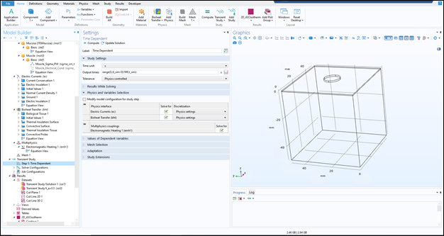
• Assign the desired output times under Transient Study and Step 1: Time Dependent.
  When initially setting up and testing the simulation an output animation is helpful for debugging. A series of output times is required for setting up an output animation. In the case below, 1000 outputs times evenly spaced over the entire simulation time were selected. To do this input "range(0,(t_sim-0)/999,t_sim)".  If the user requires only a single output time or animation over a portion of the simulation, this field can be modified as such.
• When the simulation setup is configured as desired click Compute. A progress bar will display in the bottom right of the screen. If desired, display the progress window to monitor the simulation while solving.

9. Visualizing Results

In this section, a series of visualization options are provided. When the simulation is finished, the user must set up the desired visualization techniques. 

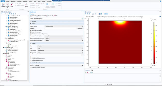
A. D43 vs Time

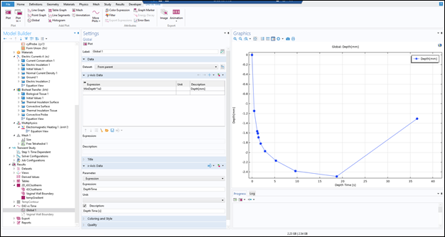
This visualization uses the conditional variables input during simulation setup to plot the approximate depth of a 43C isotherm throughout the entire simulation.

• Make a 1D plot group by right clicking on Results then 1D Plot Group. 
• Right click the new 1D Plot Group and select a Global Plot and assign the y-axis expression to "MinDepth*1e3". This corresponds to the depth of the 43C isotherm. The resultant plot should appear as below. Note: the output of this plot depends heavily on the resolution of the mesh.

B. Isothermal Line and Thermal Contour

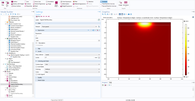
• To visualize the thermal field within the geometry the user can use this visualization as a starting point. Right click Results and select 2D Plot Group.
• Add a contour line indicating the depth of the outer bound of the vaginal wall (in this case 2.7mm) by right clicking 2D Plot Group then Contour and assigning the variables as below.

• Next add a second contour using the same method as above and assign the Expression to T and the Levels to 43 in unit degC. This one should be set to a high contrast color for visibility.

• Finally set surface to show Temperature in degC by right clicking 2D Plot Group then Surface then input the values as below. In this visualization we use the ThermalLight color table.

10. Animations

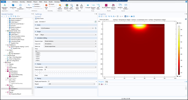
Animations can be helpful to understand the temporal progression of the 43C isotherm as well as the temperature field throughout the domain. This section demonstrates making an animation of the thermal contour visualization in the prior section.

• Right click Export and select Animation and configure as such

11. Exporting Results

Any of the above visualizations can be exported by right clicking the plot group and selecting Add Image to Export then under the Export level in the Model Builder then configuring and exporting to file.

A. Exporting a COMSOL Report

If the user wants explicit record of the simulation and setup, export a report in COMSOL.

• Right click Report, select the level of detail desired, click the Generate button with the settings below or modified as desired.

B. Suggested Use of Results

This simulation technique provides a screening-level check of the depth of thermal dispersion of a monopolar RF vaginal thermotherapy device. The results of the simulation may inform users as to what input parameters may heat past the vaginal wall, unintentionally affecting nearby tissue structures. The user may use this technique to iteratively adjust input parameters and check results against the model. This analysis may be used to inform the range of parameters used in subsequent in vitro, animal, or clinical studies of the device.

12. Validation

The model has been validated comparting with results with literature studies by Franco et al (2009) and Franco et al (2010). In the validation procedure, some parameters of the model were modified to match the validation case. The dimensions of the model, the material properties assigned to the tissue layers, and the input parameters were all modified to match the comparator. Some of the model details, namely, boundary condition, initial conditions, computational mesh statistics, and implementation of some input parameters, were not included in the comparator documentation. From this visual test, the model output behaves similarly to the experimental results.

W. Franco, A. Kothare, S. J. Ronan, R. C. Grekin and T. H. McCalmont, "Hyperthermic Injury to Adipocyte Cells by Selective Heating of Subcutaneous Fat With a Novel Radiofrequency Device: Feasibility Studies," Lasers in Surgery and Medicine, vol. 42, pp. 361-370, 2010.

W. Franco, A. Kothare and D. J. Goldberg, "Controlled Volumetric Heating of Subcutaneous Adipose Tissue Using a Novel Radiofrequency Technology," Lasers in Surgery and Medicine, vol. 41, pp. 745-750, 2009.

Please note that, additional verification, validation, and uncertainty quantification (VVUQ) will be needed depending on the model risk and how the model is used in combination other pre-clinical in vitro or in vivo test methods. Additional details about VVUQ requirements and credibility assessment is provided in the ASME V&V 40-2018 standard.

COMSOL Inc. has performed numerous verification studies on various components of the software. These verification studies have been documented: Verification and Validation Models Using COMSOL Software.

Bioheat transfer validation study performed with COMSOL Multiphysics:

M. J. Rivera, J. A. López Molina, M. Trujillo, V. Romero-García and E. J. Berjano, "Analytical validation of COMSOL Multiphysics for theoretical models of Radiofrequency ablation including the Hyperbolic Bioheat transfer equation," 2010 Annual International Conference of the IEEE Engineering in Medicine and Biology, 2010, pp. 3214-3217, doi: 10.1109/IEMBS.2010.5627405.

Step by step documentation of a similar RF exposure and bioheat transfer study performed in COMSOL Multiphysics:

Amira S. Ashour, Yanhui Guo, Waleed S. Mohamed,
6 - COMSOL Multiphysics software for ablation system simulation,
Editor(s): Amira S. Ashour, Yanhui Guo, Waleed S. Mohamed,
Thermal Ablation Therapy, Academic Press, 2021, Pages 221-289, ISBN 9780128195444, https://doi.org/10.1016/B978-0-12-819544-4.00007-1.